Youth Unemployment prediction in SA

Introduction

Youth unemployment and under-employment is a major concern for any developing country, and serves as an important predictor of economic health and prosperity. Being able to predict, and understand, which young people will find employment and which ones will require additional help, helps promote evidence-based decision-making, supports economic empowerment, and allows young people to thrive in their chosen careers.

The objective of this challenge is to build a machine learning model that predicts youth employment, based on data from labour market surveys in South Africa.

This solution will help organisations like Predictive Insights achieve a baseline prediction of young peoples’ employment outcomes, allowing them to design and test interventions to help youth make a transition into the labour market or to improve their earnings.

Data

The data for this challenge comes from four rounds of a survey of youth in the South African labour market, conducted at 6-month intervals. The survey contains numerical, categorical and free-form text responses. You will also receive additional demographic information such as age and information about school level and results.

Each person in the dataset was surveyed one year prior (the ‘baseline’ data) to the follow-up survey. We are interested in predicting whether a person is employed at the follow-up survey based on their labour market status and other characteristics during the baseline.

The training set consists of one row or observation per individual - information collected at baseline plus only the Target outcome (whether they were employed or not) one year later. The test set consists of the data collected at baseline without the Target outcome.

The objective of this challenge is to predict whether a young person will be employed, one year after the baseline survey, based on their demographic characteristics, previous and current labour market experience and education outcomes, and to deliver an easy-to-understand and insightful solution to the data team at Predictive Insights.

Load libraries and data sets

library(tidyverse)
library(tidymodels)
library(xgboost)
library(bonsai)
library(treesnip)
library(catboost)
library(earth)
library(baguette)
library(dataxray)
library(finetune)
library(fastDummies)
library(themis)
library(probably)
library(corrr)
library(janitor)
library(dlookr)
library(DataExplorer)
library(mice)
library(skimr)
library(here)
library(gt)
library(DT)
library(patchwork)

The dimensions of our training set are:  4020 21 
The dimensions of the testing set are:  1934 20

The table below gives us a quick view at the training dataset.

Data Exploration

I am going to explore the training and testing sets to uncover any potential quality issue.

Data summary

Name	df_train
Number of rows	4020
Number of columns	21
_______________________
Column type frequency:
character	9
Date	1
numeric	11
________________________
Group variables	None

Variable type: character

skim_variable	n_missing	complete_rate	min	max	empty	n_unique	whitespace
person_id	0	1.00	13	13	0	4020	0
status	0	1.00	5	22	0	7	0
geography	0	1.00	5	6	0	3	0
province	0	1.00	7	13	0	9	0
math	3023	0.25	8	10	0	7	0
mathlit	2667	0.34	8	10	0	7	0
additional_lang	2002	0.50	9	10	0	6	0
home_lang	3639	0.09	9	10	0	6	0
science	3288	0.18	8	10	0	7	0

Variable type: Date

skim_variable	n_missing	complete_rate	min	max	median	n_unique
survey_date	0	1	2021-08-11	2023-03-27	2022-09-03	79

Variable type: numeric

skim_variable	n_missing	complete_rate	mean	sd	p0	p25	p50	p75	p100	hist
round	0	1.00	3.13	0.98	1	2	3	4	4	▁▃▁▃▇
tenure	1394	0.65	582.88	621.22	0	95	395	819	3560	▇▂▁▁▁
matric	1008	0.75	0.85	0.36	0	1	1	1	1	▂▁▁▁▇
degree	1831	0.54	0.08	0.27	0	0	0	0	1	▇▁▁▁▁
diploma	1809	0.55	0.08	0.27	0	0	0	0	1	▇▁▁▁▁
schoolquintile	1661	0.59	2.70	1.32	0	2	3	4	5	▆▆▇▃▃
female	0	1.00	0.56	0.50	0	0	1	1	1	▆▁▁▁▇
sa_citizen	0	1.00	1.00	0.02	0	1	1	1	1	▁▁▁▁▇
birthyear	0	1.00	1997.46	4.38	1972	1995	1999	2000	2004	▁▁▂▃▇
birthmonth	0	1.00	5.34	3.81	1	1	5	9	12	▇▃▂▃▃
target	0	1.00	0.27	0.44	0	0	0	1	1	▇▁▁▁▃

Is there any duplicate observation?

# A tibble: 0 × 22
# ℹ 22 variables: person_id <chr>, survey_date <date>, round <dbl>,
#   status <chr>, tenure <dbl>, geography <chr>, province <chr>, matric <dbl>,
#   degree <dbl>, diploma <dbl>, schoolquintile <dbl>, math <chr>,
#   mathlit <chr>, additional_lang <chr>, home_lang <chr>, science <chr>,
#   female <dbl>, sa_citizen <dbl>, birthyear <dbl>, birthmonth <dbl>,
#   target <dbl>, dupe_count <int>

No duplicated value.

Let us have a glimpse of our training data set

Rows: 4,020
Columns: 21
$ person_id       <chr> "Id_eqz61wz7yn", "Id_kj5k3g5wud", "Id_9h0isj38y4", "Id…
$ survey_date     <date> 2022-02-23, 2023-02-06, 2022-08-08, 2022-03-16, 2023-…
$ round           <dbl> 2, 4, 3, 2, 4, 4, 4, 4, 4, 4, 3, 2, 1, 1, 2, 1, 3, 2, …
$ status          <chr> "studying", "unemployed", "other", "unemployed", "stud…
$ tenure          <dbl> NA, 427, NA, 810, NA, NA, 1826, 462, 273, 1859, NA, 73…
$ geography       <chr> "Rural", "Suburb", "Urban", "Urban", "Urban", "Rural",…
$ province        <chr> "Mpumalanga", "North West", "Free State", "Eastern Cap…
$ matric          <dbl> 1, 1, 1, NA, NA, NA, 1, 0, 1, NA, 1, 1, 1, 0, 1, 1, 1,…
$ degree          <dbl> 0, 0, 0, NA, NA, NA, 0, 0, NA, NA, NA, NA, NA, NA, NA,…
$ diploma         <dbl> 0, 0, 0, NA, NA, NA, 0, 0, NA, NA, NA, NA, NA, NA, NA,…
$ schoolquintile  <dbl> 3, 1, NA, NA, NA, NA, 2, 3, 1, NA, 2, 1, 4, 1, NA, 3, …
$ math            <chr> "0 - 29 %", "30 - 39 %", "30 - 39 %", NA, NA, NA, "30 …
$ mathlit         <chr> NA, NA, NA, NA, NA, NA, NA, NA, NA, NA, NA, NA, NA, NA…
$ additional_lang <chr> "50 - 59 %", "40 - 49 %", "40 - 49 %", NA, NA, NA, "60…
$ home_lang       <chr> NA, NA, NA, NA, NA, NA, NA, NA, NA, NA, NA, NA, NA, NA…
$ science         <chr> "0 - 29 %", "30 - 39 %", "30 - 39 %", NA, NA, NA, "40 …
$ female          <dbl> 1, 1, 0, 0, 1, 1, 1, 0, 0, 0, 1, 1, 0, 0, 0, 1, 0, 0, …
$ sa_citizen      <dbl> 1, 1, 1, 1, 1, 1, 1, 1, 1, 1, 1, 1, 1, 1, 1, 1, 1, 1, …
$ birthyear       <dbl> 2000, 1989, 1996, 2000, 1998, 1996, 2000, 1997, 2000, …
$ birthmonth      <dbl> 5, 4, 7, 1, 12, 12, 1, 1, 1, 4, 9, 3, 9, 12, 12, 11, 5…
$ target          <dbl> 0, 1, 1, 0, 0, 0, 0, 0, 0, 1, 1, 0, 1, 0, 0, 1, 1, 1, …

Let us first do some data cleaning as the nature and formatting of the data can influence the results of some EDA search.

0 = No: Person is unemployed

1 =Yes: Person is employed

### Train data
train_cleaned <- df_train %>% 
  mutate(target = as.factor(case_when(
    target == 0 ~ "No",
    target == 1 ~ "Yes",
    TRUE ~ NA), ordered = FALSE)) %>% 
  mutate_at(c(8:10), ~ as.factor(case_when(.== 0 ~ "No",
                                  .== 1 ~ "Yes",
                                  TRUE ~ NA), ordered = FALSE)) %>% 
  mutate_if(is.character, as.factor, ordered = FALSE) %>% 
  mutate(gender = as.factor(case_when(
    female == 1 ~ "F",
    female == 0 ~ "M")
  ),
    .keep = "unused", ordered = FALSE) %>% 
  mutate_at(c(3,11),  as.factor, ordered = FALSE) %>% 
  mutate(Year_survey = year(survey_date), .keep = "unused") %>% 
  mutate(age = Year_survey - birthyear) %>% 
  select(-c(sa_citizen,person_id)) 

### Test data
test_cleaned <- df_test %>% 
  mutate_at(c(8:10), ~ as.factor(case_when(.== 0 ~ "No",
                                  .== 1 ~ "Yes",
                                  TRUE ~ NA), ordered = FALSE)) %>% 
  mutate_if(is.character, as.factor, ordered = FALSE) %>% 
  mutate(gender = as.factor(case_when(
    female == 1 ~ "F",
    female == 0 ~ "M")
  ),
    .keep = "unused", ordered = FALSE) %>% 
  mutate_at(c(3,11),  as.factor, ordered = FALSE) %>% 
  mutate(Year_survey = year(survey_date), .keep = "unused") %>% 
  mutate(age = Year_survey - birthyear) %>% 
  select(-c(sa_citizen,person_id)) 

What are some quality issues observed in numerical data ?

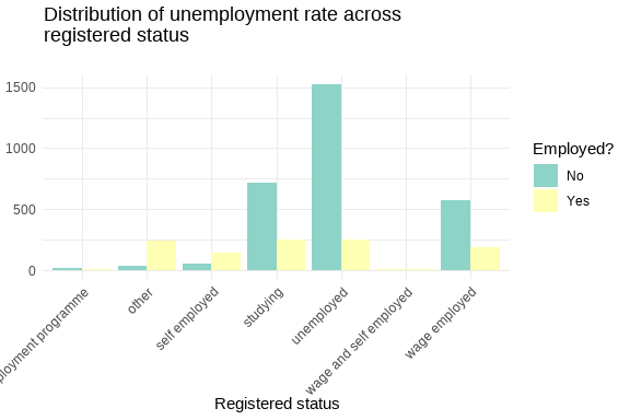
How does the target variable relate to the status variable?

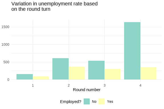
How do variables correlate?

Here I convert all factor variable to numerical variables and then apply correlation for further investigation.

below is a tibble of correlation values larger and lower than 0.25 based on the `pearson` correlation.

Key findings:

• Those who perform well in Math are correlated to those who performed well in Home_language.

• There is a high correlation between the missing values under degree and diploma; but also those in matric.

• There is a strong correlation in the performance in Science and Math as seen in the above table.

How does holding whether a post-matric qualification (diploma and/or a degree) influence the unemployment rate?

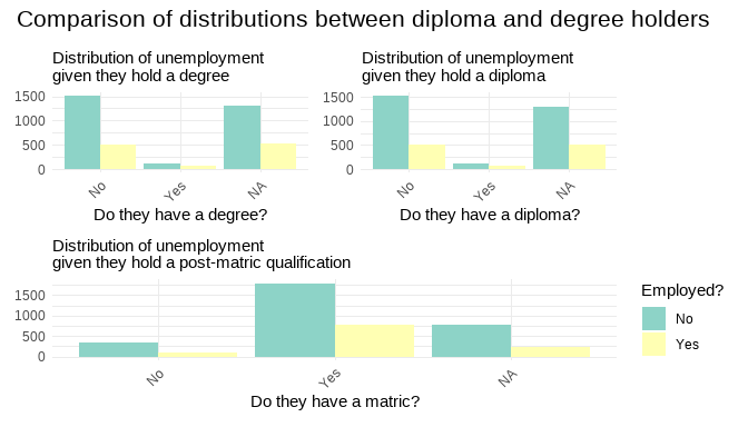
We observe a clear relationship between the two distribution from the degree and diploma holders.

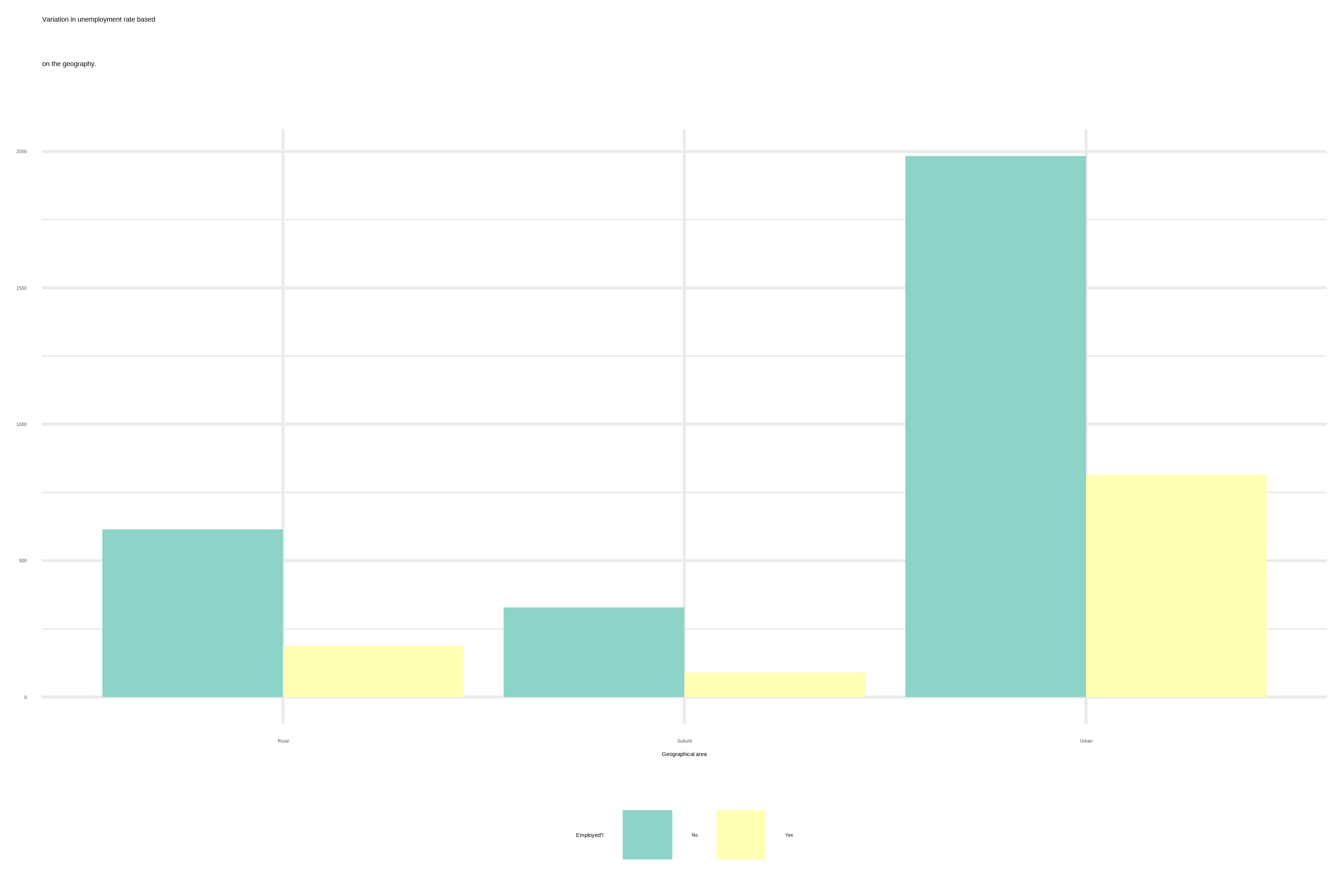
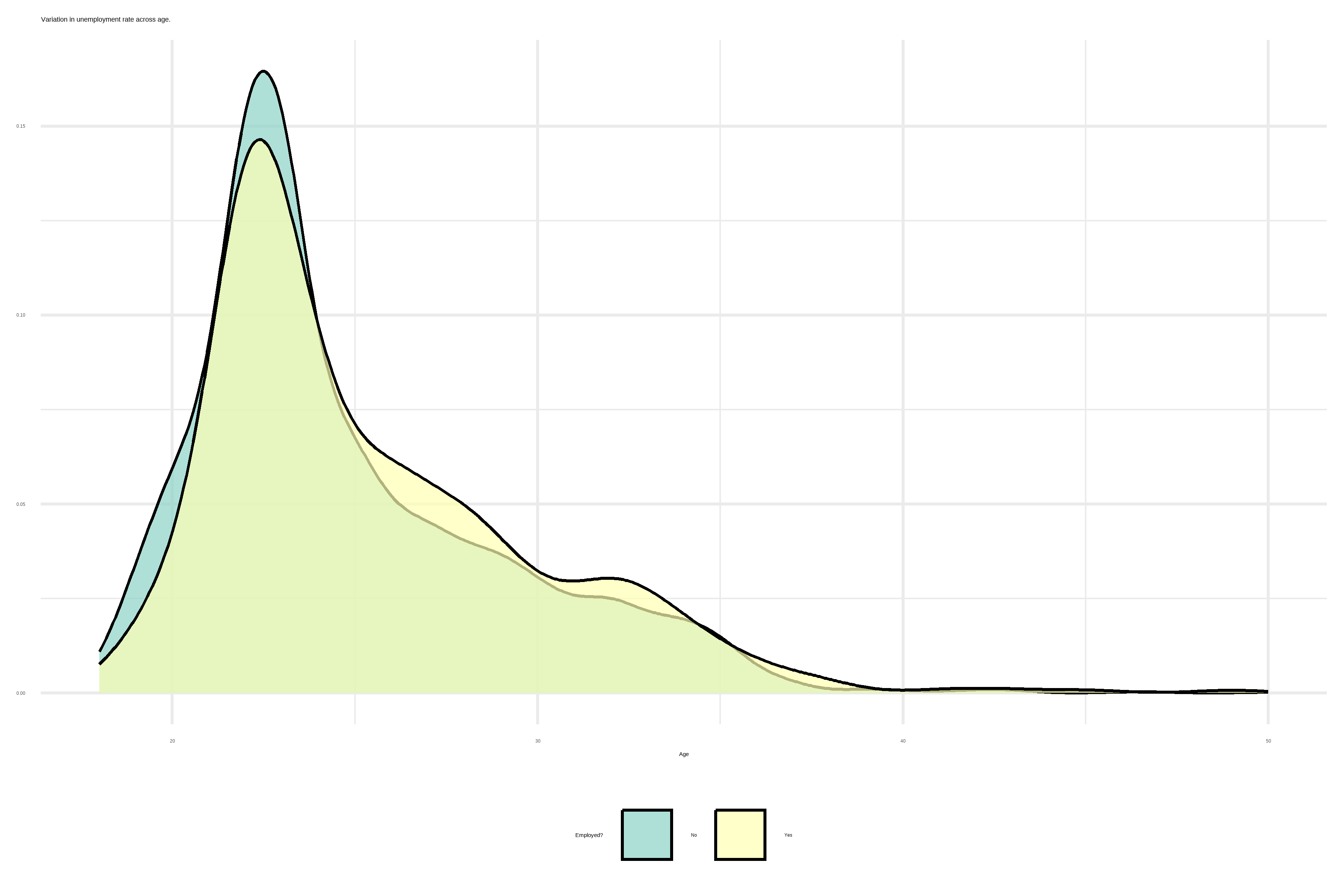
We observe that not only most of our observations come from urban areas and those from rural and suburb areas are minority in this study.

Feature Engineering

Some feature engineering that I want to apply and see the results on the performance:

• Reduce the levels in the status variable and remain with 3 levels instead of 7; same with the geography variable to remain with only 2 geographical areas instead of the 3 we currently have;

• As both the matric and degree variables follow the same distribution, combine them into a single one or only select one namely post-matric;

• Both Math and Mathlit have a high percentage of NAs, 75% and 66% respectively. However, most of the time, whenever an instance has a value in one, it doesn’t have in the other. So I will combine both variables into math which should reduce/remove the number NAs while reducing the number of feature;

  I will also do the same for the variable additional_lang and home_lang;

  Furthermore, I will group marks into 2 : fail and pass.

• As for the schoolquintile variable, we know from research that could separate them into two groups: non-fee schools (Q1, Q2, and Q3) and affluent schools (Q4 and Q5).

• Levels in status can be grouped together to only form 4 distinct levels: unemployed, employed(wage employed, self employed, wage and self employed, and employment programme), student, and other.

So let’s us do it!

## TRAIN set feature engineering -------------------------
train <- train_cleaned %>% 
  mutate(math = as.factor(case_when(
    is.na(math) & is.na(mathlit) ~ NA,
    is.na(math) & !is.na(mathlit) ~ mathlit,
    !is.na(math) & is.na(mathlit) ~ math,
    TRUE ~ paste(math, mathlit)
  )), .keep = "unused", ordered = FALSE) %>% 
  mutate(math =as.factor(case_when(
    math %in% c("0 - 29 %","30 - 39 %","40 - 49 %") ~ "fail",
    math %in% c("50 - 59 %","60 - 69 %",
                "70 - 79 %","80 - 100 %") ~ "pass")), ordered = FALSE) %>% 
  mutate(language = as.factor(case_when(
    is.na(home_lang) & is.na(additional_lang) ~ NA,
    is.na(home_lang) & !is.na(additional_lang) ~ additional_lang,
    !is.na(home_lang) & is.na(additional_lang) ~ home_lang,
    TRUE ~ paste(home_lang, additional_lang)
  )), .keep = "unused", ordered = FALSE) %>% 
  mutate(language = as.factor(case_when(
    language %in% c("30 - 39 %","40 - 49 %") ~ "fail",
    language %in% c("50 - 59 %","60 - 69 %","70 - 79 %",
                    "80 - 100 %") ~ "pass"
  )), ordered = FALSE) %>% 
  mutate(geography = as.factor(case_when(
    geography == "Urban" ~ "Urban",
    geography == "Rural" ~ "Rural",
    geography == "Suburb" ~ "Rural")), ordered = FALSE) %>% 
  mutate(post_matric = as.factor(case_when(
    is.na(degree) & is.na(diploma) ~ NA,
    is.na(degree) & !is.na(diploma) ~ diploma,
    !is.na(degree) & is.na(diploma) ~ degree,
    degree == "Yes" & diploma == "Yes" ~ "Yes",
    degree == "No" & diploma == "No" ~ "No",
    degree == "Yes" & diploma == "No" ~ "Yes",
    degree == "No" & diploma == "Yes" ~ "Yes"))
    ,.keep = "unused", ordered = FALSE) %>% 
  mutate(schoolquintile = as.factor(case_when(
    schoolquintile == "0" ~ NA_character_,
    schoolquintile %in% c("1", "2", "3") ~ "no_fee",
    schoolquintile %in% c("4", "5") ~ "affluent"
    )), ordered = FALSE) %>% 
  mutate(status = as.factor(case_when(
    status == "unemployed" ~ "unemployed",
    status == "wage employed" ~ "employed",
    status == "self employed" ~ "employed",
    status == "wage and self employed" ~ "employed",
    status == "employment programme" ~ "employed",
    status == "studying" ~ "student",
    status == "other" ~ "other"
  )), ordered = FALSE) %>% 
  select(target, everything()) %>%
  mutate(target = fct_rev(target)) %>% 
  select(-c("birthmonth", "birthyear", "Year_survey"))

## TEST set feature engineering -----------------------
test <- test_cleaned %>% 
  mutate(math = as.factor(case_when(
    is.na(math) & is.na(mathlit) ~ NA,
    is.na(math) & !is.na(mathlit) ~ mathlit,
    !is.na(math) & is.na(mathlit) ~ math,
    TRUE ~ paste(math, mathlit)
  )), .keep = "unused", ordered = FALSE) %>% 
  mutate(math =as.factor(case_when(
    math %in% c("0 - 29 %","30 - 39 %","40 - 49 %") ~ "fail",
    math %in% c("50 - 59 %","60 - 69 %",
                "70 - 79 %","80 - 100 %") ~ "pass")), ordered = FALSE) %>% 
  mutate(language = as.factor(case_when(
    is.na(home_lang) & is.na(additional_lang) ~ NA,
    is.na(home_lang) & !is.na(additional_lang) ~ additional_lang,
    !is.na(home_lang) & is.na(additional_lang) ~ home_lang,
    TRUE ~ paste(home_lang, additional_lang)
  )), .keep = "unused", ordered = FALSE) %>% 
  mutate(language = as.factor(case_when(
    language %in% c("30 - 39 %","40 - 49 %") ~ "fail",
    language %in% c("50 - 59 %","60 - 69 %","70 - 79 %",
                    "80 - 100 %") ~ "pass"
  )), ordered = FALSE) %>% 
  mutate(geography = as.factor(case_when(
    geography == "Urban" ~ "Urban",
    geography == "Rural" ~ "Rural",
    geography == "Suburb" ~ "Rural")), ordered = FALSE) %>% 
  mutate(post_matric = as.factor(case_when(
    is.na(degree) & is.na(diploma) ~ NA,
    is.na(degree) & !is.na(diploma) ~ diploma,
    !is.na(degree) & is.na(diploma) ~ degree,
    degree == "Yes" & diploma == "Yes" ~ "Yes",
    degree == "No" & diploma == "No" ~ "No",
    degree == "Yes" & diploma == "No" ~ "Yes",
    degree == "No" & diploma == "Yes" ~ "Yes"))
    ,.keep = "unused", ordered = FALSE) %>% 
  mutate(schoolquintile = as.factor(case_when(
    schoolquintile == "0" ~ NA_character_,
    schoolquintile %in% c("1", "2", "3") ~ "no_fee",
    schoolquintile %in% c("4", "5") ~ "affluent"
    )), ordered = FALSE) %>% 
  mutate(status = as.factor(case_when(
    status == "unemployed" ~ "unemployed",
    status == "wage employed" ~ "employed",
    status == "self employed" ~ "employed",
    status == "wage and self employed" ~ "employed",
    status == "employment programme" ~ "employed",
    status == "studying" ~ "student",
    status == "other" ~ "other"
  )), ordered = FALSE) %>% 
  select(-c("birthmonth", "birthyear", "Year_survey"))

Let us now re-examine our newly engineered dataset:

How are the missing value looking like now:

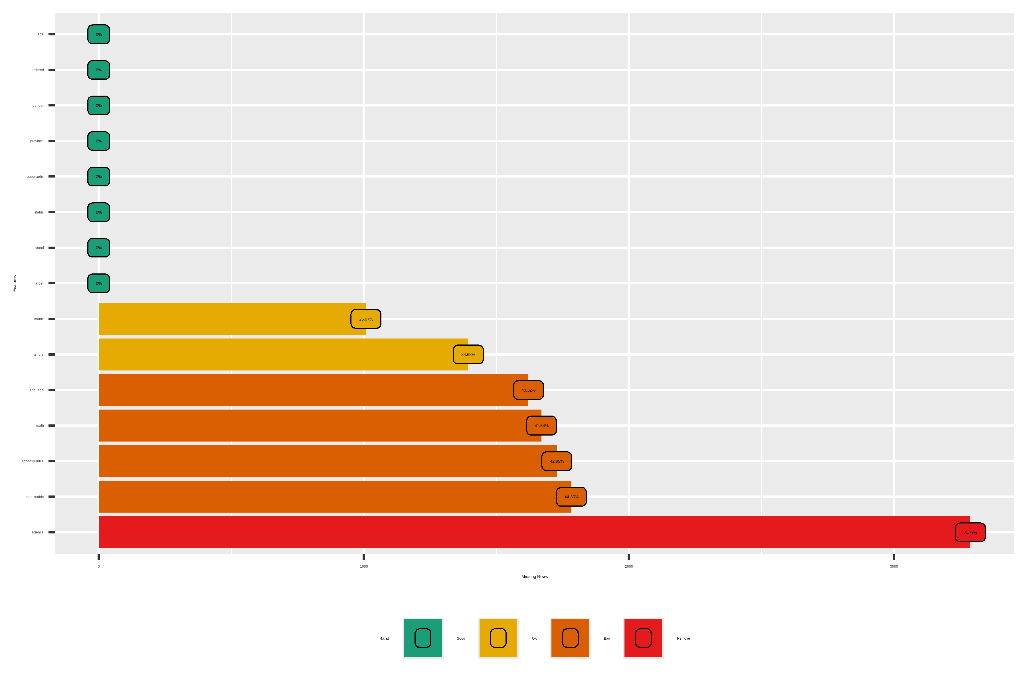
• We can see that the science variable ought to be removed as it is mostly missing in the data set.

• We have to deal with the schoolquintile variable which is missing 43% of the time as well as matric and tenure variables. Or maybe just make use of a model robust to missing values.

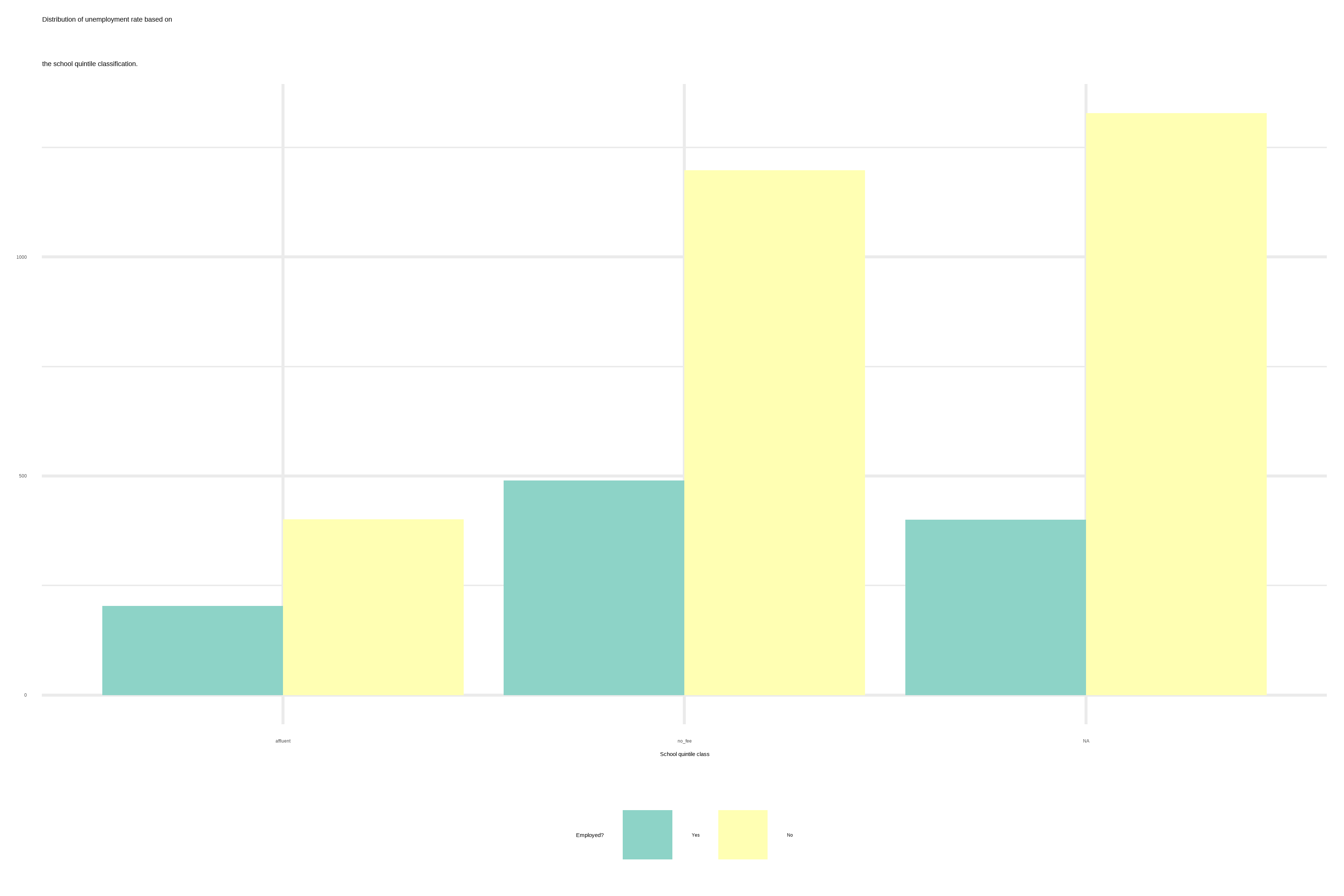
We observe that we have more people in no-fee schools than in affluent schools, but also that the ratio of unemployment is way bigger in no-fee schools than the affluent schools.

What variables are skewed?

[1] "tenure" "age"   

Using the package DataExplorer, I impute NAs in tenure, schoolquintile, matric, language, math, and post_matric variables through the `mice` method:

schoolquintile_imputed <- imputate_na(train, 
                      schoolquintile,
                      target, 
                      method = "mice",
                      seed = 2024)

tenure_imputed <- imputate_na(train, 
                      tenure,
                      target, 
                      method = "mice",
                      seed = 2024)

matric_imputed <- imputate_na(train, 
                      matric,
                      target, 
                      method = "mice",
                      seed = 2024)

language_imputed <- imputate_na(train, 
                        language,
                        target, 
                        method = "rpart"
                        )

math_imputed <- imputate_na(train, 
                      math,
                      target, 
                      method = "mice",
                      seed = 2024)

post_matric_imputed <- imputate_na(train, 
                      post_matric,
                      target, 
                      method = "mice",
                      seed = 2024)

p1 <- plot(schoolquintile_imputed) + ggtitle("School quintile") 
p2 <- plot(matric_imputed) + ggtitle("Matric") 
p3 <- plot(math_imputed) + ggtitle("Math") 
p4 <- plot(tenure_imputed) + ggtitle("Tenure") 
p5 <- plot(language_imputed) + ggtitle("Language") 
p6 <- plot(post_matric_imputed) + ggtitle("Post matric") 



p1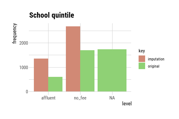

p2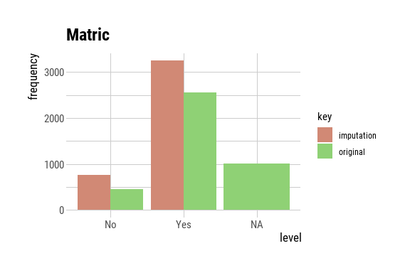

p3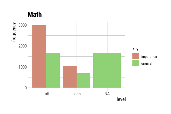

p4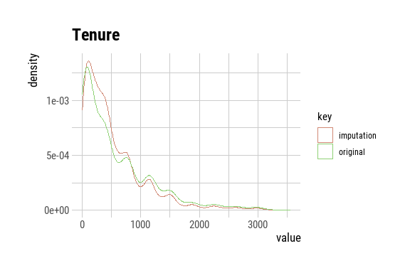

p5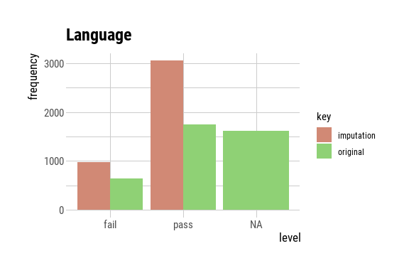

p6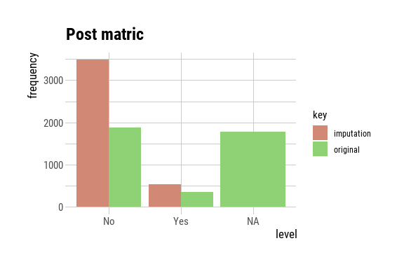

Modeling

Now we can start with the modeling phase.

Define models

### LOGISTIC REGRESSION ---------------
lr_spec <- logistic_reg(mixture = tune(), penalty = tune()) %>% 
  set_engine("glmnet") %>% 
  set_mode("classification")


### CatBoost ---------------
cat_spec <- boost_tree(trees = 1000,
                            min_n = tune(),
                            learn_rate = tune(),
                            tree_depth = tune()
                            ) %>% 
  set_engine("catboost", nthread = 4) %>% 
  set_mode("classification")
### Random forest---------------
rf_spec <- 
  rand_forest(
    mtry = tune(),
    min_n = tune(),
    trees = 1000
  ) %>%
  set_mode("classification") %>%
  set_engine("ranger")

### SUPPORT VECTOR MACHINE ---------------

svm_spec <- svm_rbf("classification",
                    cost = tune(),
                    rbf_sigma = tune(),
                    margin = tune()) %>% 
  set_engine("kernlab")
### MARS Model -------------------

bag_spec <- bag_mars("classification",
                     num_terms = tune(),
                     prod_degree = tune()) %>%
  set_engine("earth")

Now I will write some recipes

Define recipes

library(themis)
#### Data budget ------------


## Bind imputed variables to the original training data
train_full <- train %>% 
  mutate(language_imputed = language_imputed,
         math_imputed = math_imputed,
         matric_imputed = matric_imputed,
         post_matric_imputed = post_matric_imputed,
         schoolquintile_imputed = schoolquintile_imputed,
         tenure_imputed = tenure_imputed)

### We have both imputed and non-imputed variables
set.seed(2024)
splits <- initial_split(train_full, strata = target)
training <- training(splits)
testing <- testing(splits)


##### training folds ----------
set.seed(2024)
folds <- bootstraps(training, times = 30)



### Basic recipe: ----------
## Full imputation,
## Dummify,
## transform,
## normalize,
## upsample imbalance

basic_rec <- recipe(target ~., data = training) %>% 
  step_rm(post_matric,math,language,matric,
            tenure,schoolquintile,science) %>%
  step_dummy(all_nominal_predictors(),
             -all_outcomes()) %>%
  step_nzv(all_predictors()) %>% 
  step_YeoJohnson(c("tenure_imputed","age")) %>% 
  step_corr(all_numeric_predictors(),threshold = tune("cor_thresh_base")) %>%
  step_normalize(all_numeric_predictors(),
                 -all_outcomes()) %>% 
  step_smote(target, over_ratio = 0.8)

## Making sure the recipe works as intended
# basic_rec %>% prep(training) %>% juice()

Models training

Now we train our models

### Elastic net workflow
lr_wflow <- workflow() %>% 
  add_model(lr_spec) %>% 
  add_recipe(basic_rec)

set.seed(2024)
lr_grid <- lr_wflow %>%
  parameters() %>%
  grid_latin_hypercube(size = 25)

### Random forest workflows

rf_wflow <- workflow() %>% 
  add_model(rf_spec) %>% 
  add_recipe(basic_rec)

set.seed(2024)
rf_params <- rf_wflow %>%
  parameters(
    mtry(range = c(1, 10)),
    trees(range = c(100, 500)),
    min_n(range = c(1, 10))
  ) 

rf_params <- finalize(rf_params, training)

rf_grid <- grid_latin_hypercube(rf_params, size = 25)


### CATBOOST
cat_wflow <- workflow() %>% 
  add_model(cat_spec) %>% 
  add_recipe(basic_rec)

cat_param <-
  cat_wflow %>% 
  parameters() %>% 
  update(
    min_n       = min_n(c(1, 10)), 
    learn_rate  = learn_rate(c(0.02, 0.2)),
    tree_depth  = tree_depth(c(4,10))
  )

### SVM 
svm_wflow <- workflow() %>% 
  add_model(svm_spec) %>% 
  add_recipe(basic_rec)

set.seed(2024)
svm_grid <- svm_wflow %>%
  parameters() %>%
  grid_latin_hypercube(size = 25)


### MARS
mars_wflow <- workflow() %>% 
  add_model(bag_spec) %>% 
  add_recipe(basic_rec)

set.seed(2024)
mars_grid <- mars_wflow %>%
  parameters() %>%
  grid_latin_hypercube(size = 25)

We have 8 cores at our disposal:

system 
     8 

Now we do the actual tuning:

##### WORKFLOW ------------
library(bonsai)
library(doParallel)
metric <- metric_set(roc_auc,mn_log_loss, accuracy)

set.seed(2024)
registerDoMC(cores = max(1, availableCores() - 1))
### Elastic net --
lr_results <- lr_wflow %>% 
  tune_race_anova(resamples = folds,
                  grid = lr_grid,
                  control = control_race(
                    verbose = TRUE,
                    verbose_elim = TRUE,
                    save_pred = TRUE,
                    save_workflow = TRUE,
                    parallel_over = "everything"))


### Random forest --
rf_results <- rf_wflow %>% 
  tune_grid(resamples = folds,
            grid = rf_grid,
            metrics = metric,
            control = control_grid(verbose = TRUE,
                                   save_pred = TRUE,
                                   save_workflow = TRUE,
                                   parallel_over = "everything"))

      
### CatBoost ---
catBoost_results <- cat_wflow %>% 
    tune_bayes(resamples = folds,
               param_info = cat_param,
               initial = 5,
               iter = 30,
               metrics = metric,
               control = control_bayes(verbose = TRUE,
                                     save_pred = TRUE,
                                     save_workflow = TRUE,
                                     parallel_over = "everything"))

### Mars ---
registerDoMC(cores = max(1, availableCores() - 1))
mars_results <- mars_wflow %>% 
    tune_race_anova(resamples = folds,
                  grid = mars_grid,
                  control = control_race(
                    verbose = TRUE,
                    verbose_elim = TRUE,
                    save_pred = TRUE,
                    save_workflow = TRUE,
                    parallel_over = "everything"))
                              
### Support Vector Machine ----
svm_results <- svm_wflow %>% 
    tune_race_anova(resamples = folds,
                  grid = svm_grid,
                  control = control_race(
                    verbose = TRUE,
                    verbose_elim = TRUE,
                    save_pred = TRUE,
                    save_workflow = TRUE,
                    parallel_over = "everything"))

# A tibble: 5 × 2
  models    names   
  <list>    <chr>   
1 <race[+]> elastic 
2 <tune[+]> rf      
3 <tune[+]> catBoost
4 <race[+]> mars    
5 <race[+]> svm     

Let us analyse the results

Elastic net results

# A tibble: 4 × 9
  penalty mixture cor_thresh_base .metric .estimator  mean     n std_err .config
    <dbl>   <dbl>           <dbl> <chr>   <chr>      <dbl> <int>   <dbl> <chr>  
1 4.23e-8   0.167           0.997 roc_auc binary     0.790    30 0.00220 Prepro…
2 9.93e-6   0.230           0.957 roc_auc binary     0.790    30 0.00220 Prepro…
3 2.28e-5   0.382           0.587 roc_auc binary     0.790    30 0.00220 Prepro…
4 3.69e-7   0.294           0.691 roc_auc binary     0.790    30 0.00220 Prepro…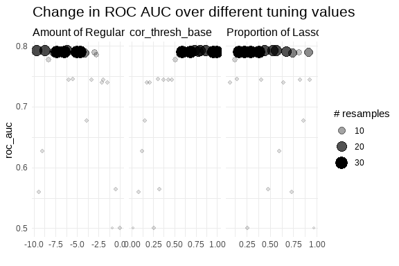

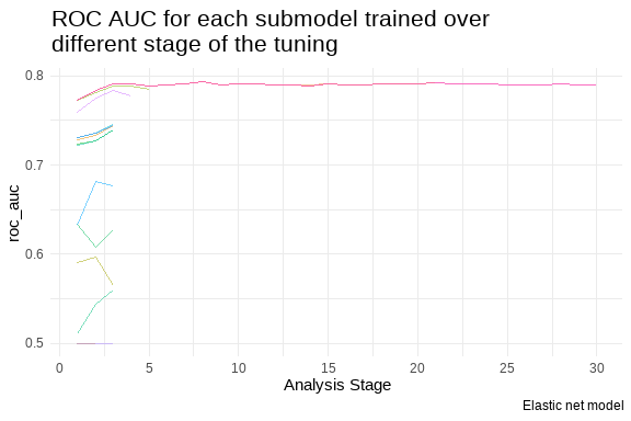
Not bad at all, we that we are approaching 80% of ROC_AUC mostly using 20 to 30 folds resamples. Maybe experimenting on increasing the number of folds.

Random Forest results

# A tibble: 5 × 9
   mtry min_n cor_thresh_base .metric .estimator  mean     n std_err .config    
  <int> <int>           <dbl> <chr>   <chr>      <dbl> <int>   <dbl> <chr>      
1    13    30           0.610 roc_auc binary     0.820    30 0.00234 Preprocess…
2    15    32           0.669 roc_auc binary     0.819    30 0.00236 Preprocess…
3    12    15           0.587 roc_auc binary     0.817    30 0.00233 Preprocess…
4     9    18           0.803 roc_auc binary     0.817    30 0.00235 Preprocess…
5     7    27           0.773 roc_auc binary     0.816    30 0.00246 Preprocess…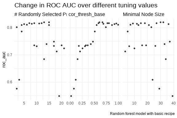

Above 15 random selected predictor, the model’s perfomance starts to decrease and the performance increases when the correlation threshold is above 50%.

CatBoost results

# A tibble: 5 × 11
  min_n tree_depth learn_rate cor_thresh_base .metric .estimator  mean     n
  <int>      <int>      <dbl>           <dbl> <chr>   <chr>      <dbl> <int>
1     9          4       1.05           0.603 roc_auc binary     0.770    30
2     6          4       1.06           0.903 roc_auc binary     0.769    30
3     8          4       1.05           0.918 roc_auc binary     0.768    30
4     8          4       1.05           0.883 roc_auc binary     0.767    30
5     8          4       1.07           0.581 roc_auc binary     0.766    30
# ℹ 3 more variables: std_err <dbl>, .config <chr>, .iter <int>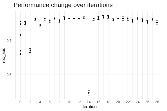

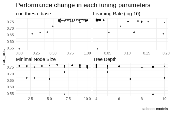
I had so much expectation for the catboost, however maybe further tuning may be required.

MARS results

# A tibble: 2 × 9
  num_terms prod_degree cor_thresh_base .metric .estimator  mean     n std_err
      <int>       <int>           <dbl> <chr>   <chr>      <dbl> <int>   <dbl>
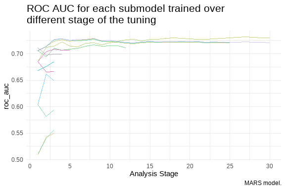
1         4           1           0.548 roc_auc binary     0.730    30 0.00484
2         5           1           0.255 roc_auc binary     0.721    30 0.00286
# ℹ 1 more variable: .config <chr>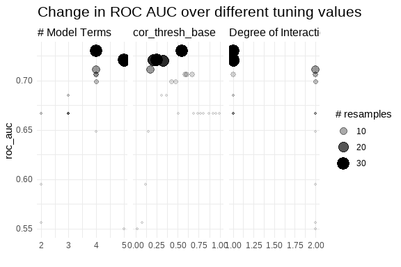

SVM results

# A tibble: 1 × 10
   cost rbf_sigma margin cor_thresh_base .metric .estimator  mean     n std_err
  <dbl>     <dbl>  <dbl>           <dbl> <chr>   <chr>      <dbl> <int>   <dbl>
1  3.11  0.000567  0.198           0.921 roc_auc binary     0.778    30 0.00252
# ℹ 1 more variable: .config <chr>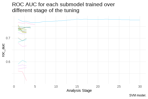

Ensemble model: Stacking

Now we will build an ensemble model using the stack package from tidymodels:

data_stack <- stacks() %>% 
  add_candidates(lr_results) %>% 
  add_candidates(catBoost_results) %>% 
  add_candidates(mars_results) %>% 
  add_candidates(rf_results) %>% 
  add_candidates(svm_results)

set.seed(2024)
model_stack <- data_stack %>% 
  blend_predictions()

library(stacks)
autoplot(model_stack)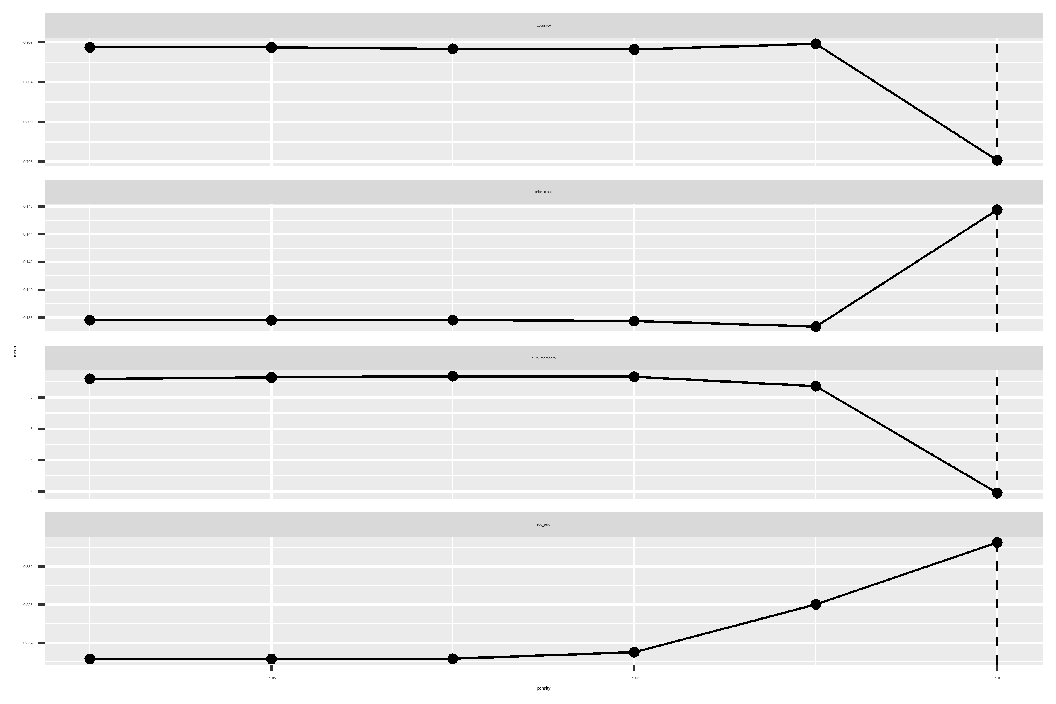

autoplot(model_stack, type = "weights")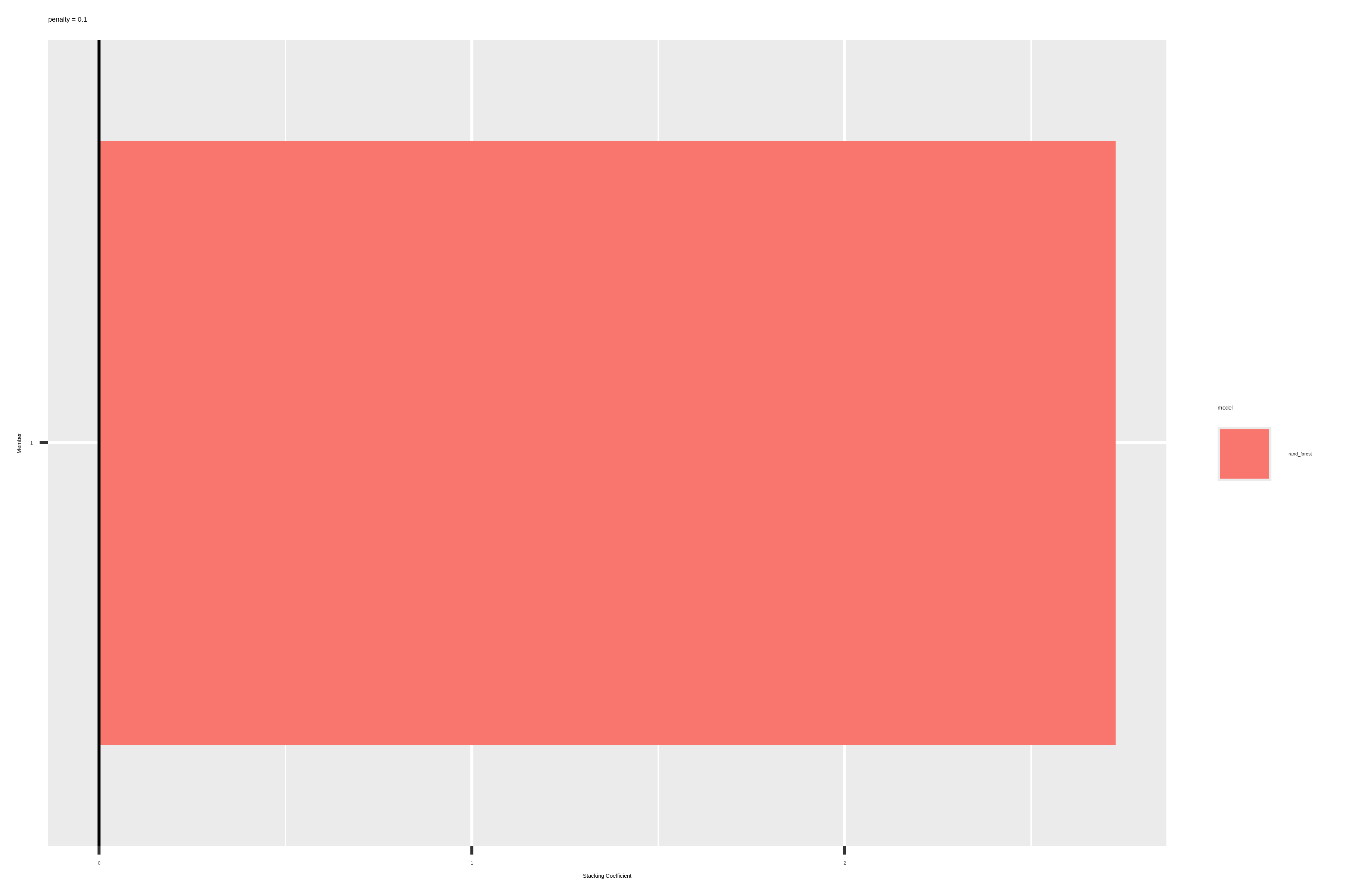

It seems that our blending decided to only keep the random forest models.

Now we train our stack model:

set.seed(2024)
stack_results <- model_stack %>% 
  fit_members()

stack_results

collect_parameters(stack_results, "rf_results")

# A tibble: 25 × 6
   member           mtry min_n cor_thresh_base terms                     coef
   <chr>           <int> <int>           <dbl> <chr>                    <dbl>
 1 rf_results_01_1     7    27          0.773  .pred_No_rf_results_01_1     0
 2 rf_results_02_1     6     7          0.997  .pred_No_rf_results_02_1     0
 3 rf_results_03_1    17    37          0.473  .pred_No_rf_results_03_1     0
 4 rf_results_04_1    19    39          0.0180 .pred_No_rf_results_04_1     0
 5 rf_results_05_1     4    21          0.870  .pred_No_rf_results_05_1     0
 6 rf_results_06_1    20    19          0.326  .pred_No_rf_results_06_1     0
 7 rf_results_07_1    15    13          0.548  .pred_No_rf_results_07_1     0
 8 rf_results_08_1     9    18          0.803  .pred_No_rf_results_08_1     0
 9 rf_results_09_1    17    26          0.180  .pred_No_rf_results_09_1     0
10 rf_results_10_1     3    24          0.117  .pred_No_rf_results_10_1     0
# ℹ 15 more rows

Let us test our stack

set.seed(2024)
stack_test_pred <- testing %>%
  bind_cols(predict(stack_results, testing, type = "prob"))

roc <- stack_test_pred %>%
  roc_auc(truth = target, .pred_Yes) %>% 
  rename(metric = .metric, estimator = .estimator, estimate = .estimate) 

roc

# A tibble: 1 × 3
  metric  estimator estimate
  <chr>   <chr>        <dbl>
1 roc_auc binary       0.828

Voilà! This project showcased that sometimes we do not need to look for ensemble models when we already have a super-saiyen model “The random forest”.

We could still try to finetune our random forest and try to squeeze out even more for an optimal value, but the winning solution was 0.86% ROC-AUC, and having 0.83% (0.8278) in our first trial is not bad at all.

Thank you for making it until the end, see you next time.