Code
library(tidyverse)
library(tidymodels)
library(xgboost)
library(dataxray)
library(finetune)
library(themis)
library(probably)
library(flextable)
library(kableExtra)
library(skimr)
library(here)
library(probably)
library(reticulate)Business value of losing a customer.
Dan A. Tshisungu
April 5, 2024
For every business to grow, they have to sustain themselves which often involves both retaining current customers and acquiring new customers. The former, however, turns out to be harder and costly. Hence the major need for every business to retain their current customers.
In this case study, I will try to predict variables to retain customers at wireless services provider called Telco. To achieve this, I will use machine learning tools to build a predictive model as well as showcase the financial implications related to the churn rate to assist Telco in preventing customers.
I will load the necessary libraries and have a look at the data we have.
The dimensions of our data set are: 7043 21Now let me check the actual data:
Rows: 7,043
Columns: 21
$ customerID       <chr> "7590-VHVEG", "5575-GNVDE", "3668-QPYBK", "7795-CFOCW…
$ gender           <chr> "Female", "Male", "Male", "Male", "Female", "Female",…
$ SeniorCitizen    <dbl> 0, 0, 0, 0, 0, 0, 0, 0, 0, 0, 0, 0, 0, 0, 0, 0, 0, 0,…
$ Partner          <chr> "Yes", "No", "No", "No", "No", "No", "No", "No", "Yes…
$ Dependents       <chr> "No", "No", "No", "No", "No", "No", "Yes", "No", "No"…
$ tenure           <dbl> 1, 34, 2, 45, 2, 8, 22, 10, 28, 62, 13, 16, 58, 49, 2…
$ PhoneService     <chr> "No", "Yes", "Yes", "No", "Yes", "Yes", "Yes", "No", …
$ MultipleLines    <chr> "No phone service", "No", "No", "No phone service", "…
$ InternetService  <chr> "DSL", "DSL", "DSL", "DSL", "Fiber optic", "Fiber opt…
$ OnlineSecurity   <chr> "No", "Yes", "Yes", "Yes", "No", "No", "No", "Yes", "…
$ OnlineBackup     <chr> "Yes", "No", "Yes", "No", "No", "No", "Yes", "No", "N…
$ DeviceProtection <chr> "No", "Yes", "No", "Yes", "No", "Yes", "No", "No", "Y…
$ TechSupport      <chr> "No", "No", "No", "Yes", "No", "No", "No", "No", "Yes…
$ StreamingTV      <chr> "No", "No", "No", "No", "No", "Yes", "Yes", "No", "Ye…
$ StreamingMovies  <chr> "No", "No", "No", "No", "No", "Yes", "No", "No", "Yes…
$ Contract         <chr> "Month-to-month", "One year", "Month-to-month", "One …
$ PaperlessBilling <chr> "Yes", "No", "Yes", "No", "Yes", "Yes", "Yes", "No", …
$ PaymentMethod    <chr> "Electronic check", "Mailed check", "Mailed check", "…
$ MonthlyCharges   <dbl> 29.85, 56.95, 53.85, 42.30, 70.70, 99.65, 89.10, 29.7…
$ TotalCharges     <dbl> 29.85, 1889.50, 108.15, 1840.75, 151.65, 820.50, 1949…
$ Churn <chr> "No", "No", "Yes", "No", "Yes", "Yes", "No", "No", "Y…Now let us explore our data
What are the summary statistics of our data?
| Name | telco_df |
| Number of rows | 7043 |
| Number of columns | 21 |
| _______________________ | |
| Column type frequency: | |
| character | 17 |
| numeric | 4 |
| ________________________ | |
| Group variables | None |
Variable type: character
| skim_variable | n_missing | complete_rate | min | max | empty | n_unique | whitespace |
|---|---|---|---|---|---|---|---|
| customerID | 0 | 1 | 10 | 10 | 0 | 7043 | 0 |
| gender | 0 | 1 | 4 | 6 | 0 | 2 | 0 |
| Partner | 0 | 1 | 2 | 3 | 0 | 2 | 0 |
| Dependents | 0 | 1 | 2 | 3 | 0 | 2 | 0 |
| PhoneService | 0 | 1 | 2 | 3 | 0 | 2 | 0 |
| MultipleLines | 0 | 1 | 2 | 16 | 0 | 3 | 0 |
| InternetService | 0 | 1 | 2 | 11 | 0 | 3 | 0 |
| OnlineSecurity | 0 | 1 | 2 | 19 | 0 | 3 | 0 |
| OnlineBackup | 0 | 1 | 2 | 19 | 0 | 3 | 0 |
| DeviceProtection | 0 | 1 | 2 | 19 | 0 | 3 | 0 |
| TechSupport | 0 | 1 | 2 | 19 | 0 | 3 | 0 |
| StreamingTV | 0 | 1 | 2 | 19 | 0 | 3 | 0 |
| StreamingMovies | 0 | 1 | 2 | 19 | 0 | 3 | 0 |
| Contract | 0 | 1 | 8 | 14 | 0 | 3 | 0 |
| PaperlessBilling | 0 | 1 | 2 | 3 | 0 | 2 | 0 |
| PaymentMethod | 0 | 1 | 12 | 25 | 0 | 4 | 0 |
| Churn | 0 | 1 | 2 | 3 | 0 | 2 | 0 |
Variable type: numeric
| skim_variable | n_missing | complete_rate | mean | sd | p0 | p25 | p50 | p75 | p100 | hist |
|---|---|---|---|---|---|---|---|---|---|---|
| SeniorCitizen | 0 | 1 | 0.16 | 0.37 | 0.00 | 0.00 | 0.00 | 0.00 | 1.00 | ▇▁▁▁▂ |
| tenure | 0 | 1 | 32.37 | 24.56 | 0.00 | 9.00 | 29.00 | 55.00 | 72.00 | ▇▃▃▃▆ |
| MonthlyCharges | 0 | 1 | 64.76 | 30.09 | 18.25 | 35.50 | 70.35 | 89.85 | 118.75 | ▇▅▆▇▅ |
| TotalCharges | 11 | 1 | 2283.30 | 2266.77 | 18.80 | 401.45 | 1397.47 | 3794.74 | 8684.80 | ▇▂▂▂▁ |
Observations:
customerID variable can be removed as it does not bring in any information to the model.
SeniorCitizen variable, currently recorded as a numeric variable should be converted to categorical.
Some variables such as InternetService, we can try to reduce the number of levels to avoid duplicate information as we have cases of Yes, No, and No internet Service, which can be combined into the level/category of No.
How does the churn rate vary across different contract types?
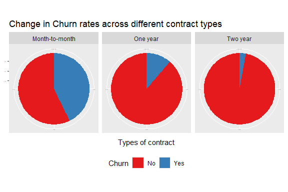
We notice here that there is a clear correlation between the duration of the contract and the decision to churn as the longer the contract, the shorter the churn rate.
What is the distribution of churn rates based on the type of internet service acquired?
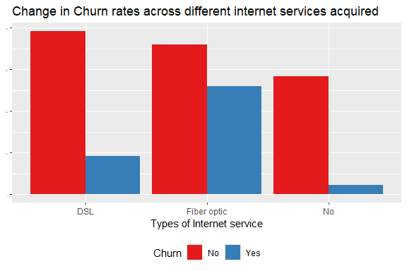
Clients who use the fiber optic are more likely to churn than other internet services.
How does the distribution of monthly charges correlate with the churn rate?
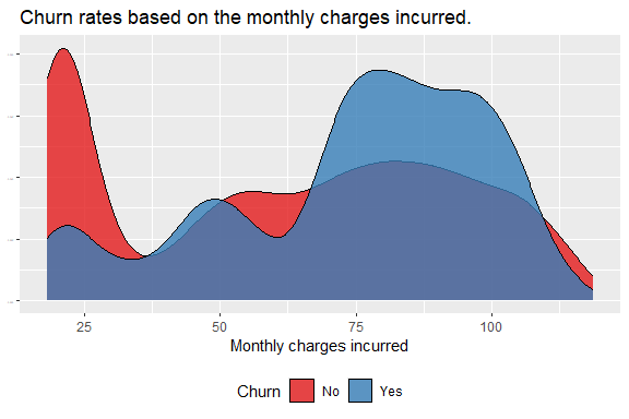
Naturally, clients experiencing high monthly charges are more like to churn.
How does the churn rate vary along the tenure period?
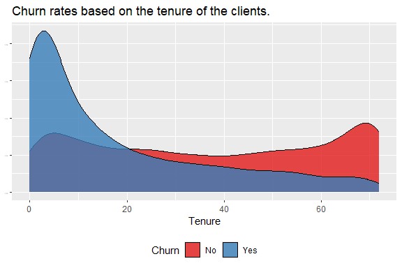
Relatively new clients are more likely to churn compared to those who have been with Telco for a longer time.
How about we check at the relationship between the monthly charges compared to the tenure of the client.
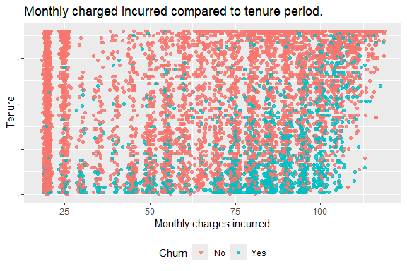
We can see that those clients who are paying the most and have a shorter tenure are more likely to churn.
The cleaning and transformations to be done:
telco_clean <- telco_df %>%
  na.omit() %>%
  mutate(Churn = fct_rev(Churn)) %>%
  mutate(SeniorCitizen = as.factor(SeniorCitizen)) %>%
  mutate_at(8, ~as.factor(case_when(.=="No phone service" ~ "No",
                                    .=="No" ~ "No",
                                    TRUE ~ "Yes"))) %>%
  mutate_at(c(10:15), ~as.factor(case_when(.=="No internet service" ~ "No",
                                    .=="No" ~ "No",
                                    TRUE ~ "Yes")))
We prepare our data for modeling
We now build our recipes for the different models depending on our choice:
I will be using an xgboost model for this case study.
I will be tuning :
max_depth
learning rate
number of estimators (trees)
I define the model, xgboost, as well as the tuning parameters below:
Boosted Tree Model Specification (classification)

Main Arguments:
  mtry = tune()
  trees = tune()
  learn_rate = tune()

Computational engine: xgboost
Then I initialise the workflow of modeling as well as the search ranges for the hyperparameters.
Now I set some metrics of interest.
I chose this time to go for a Bayesian optimization search for the tuning of the hyperparameters.
I chose 50 iterations before I like 50 cents😆, don’t fight me please
# Defining search space of the Bayesian optimisation
trade_off_decay <- function(iter) {
  expo_decay(iter, start_val = .02, limit_val = 0, slope = 1/4)
}


set.seed(2024)
xgb_results <- tune_bayes(
  xgb_wf,
  resamples = folds,
  initial   = 3,
  iter      = 50,
  metrics   = xgb_metric,
  param_info= xgb_param,
  objective = exp_improve(trade_off_decay),
  control   = control_bayes(verbose_iter = TRUE,
save_pred = TRUE))Below are the top 5 accuracy :
# A tibble: 5 × 10
   mtry trees learn_rate .metric  .estimator  mean     n std_err .config .iter
  <int> <int>      <dbl> <chr>    <chr>      <dbl> <int>   <dbl> <chr>   <int>
1     6   222       1.07 accuracy binary     0.763    10 0.00734 Iter13     13
2     8   110       1.06 accuracy binary     0.761    10 0.00630 Iter9       9
3     8   224       1.05 accuracy binary     0.761    10 0.00707 Iter11     11
4     8   114       1.23 accuracy binary     0.761    10 0.00659 Iter5       5
5     6   233       1.05 accuracy binary     0.760    10 0.00457 Iter15     15
We can clearly see that our top performer had an accuracy of 76.3% at iteration 13, followed by 76.1%, 76.1%, and 76.1% respectively at iteration 9, 11, and 5.
# A tibble: 5 × 10
   mtry trees learn_rate .metric .estimator  mean     n std_err .config .iter
  <int> <int>      <dbl> <chr>   <chr>      <dbl> <int>   <dbl> <chr>   <int>
1     7   217       1.12 roc_auc binary     0.787    10 0.00635 Iter17     17
2     8   110       1.06 roc_auc binary     0.787    10 0.00404 Iter9       9
3     6   220       1.05 roc_auc binary     0.785    10 0.00512 Iter19     19
4     5   112       1.07 roc_auc binary     0.783    10 0.00701 Iter23     23
5     7   111       1.33 roc_auc binary     0.783    10 0.00771 Iter7       7
Our best AUC, 78.7% also occured at iteration 17.
Let us how the performance fluctuated over the iterations:
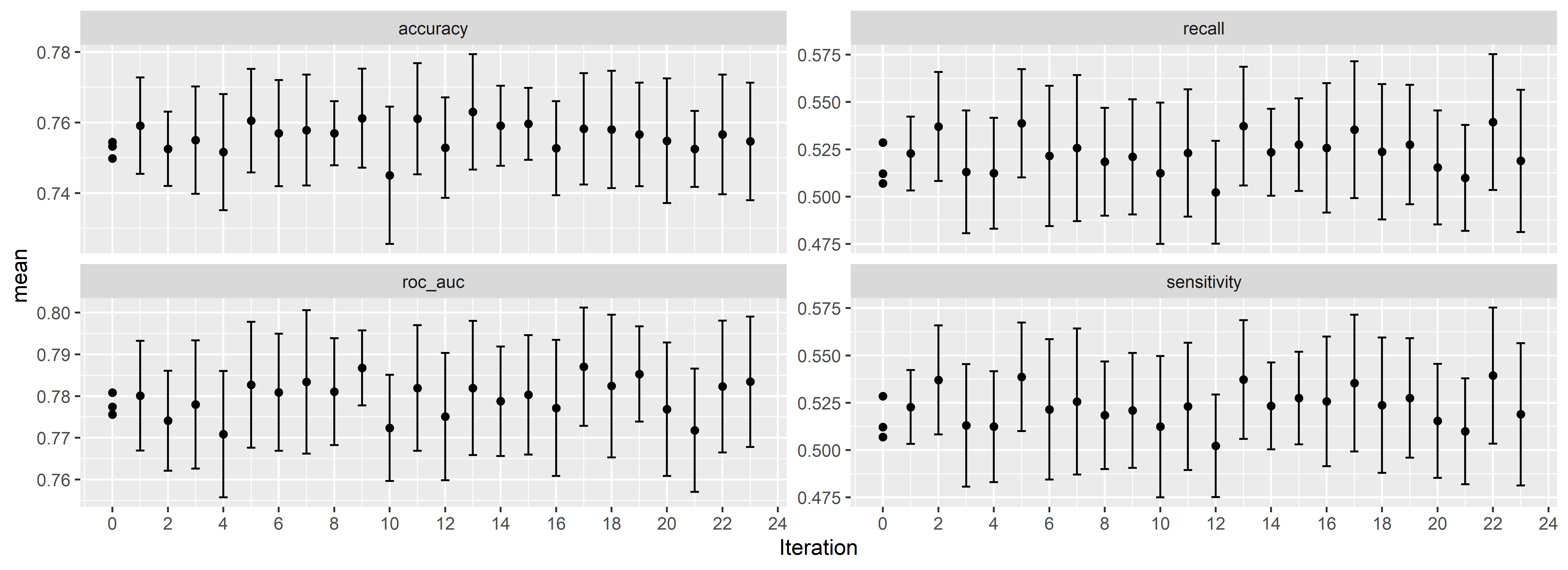
How the performaced fluctuated over the different parameters
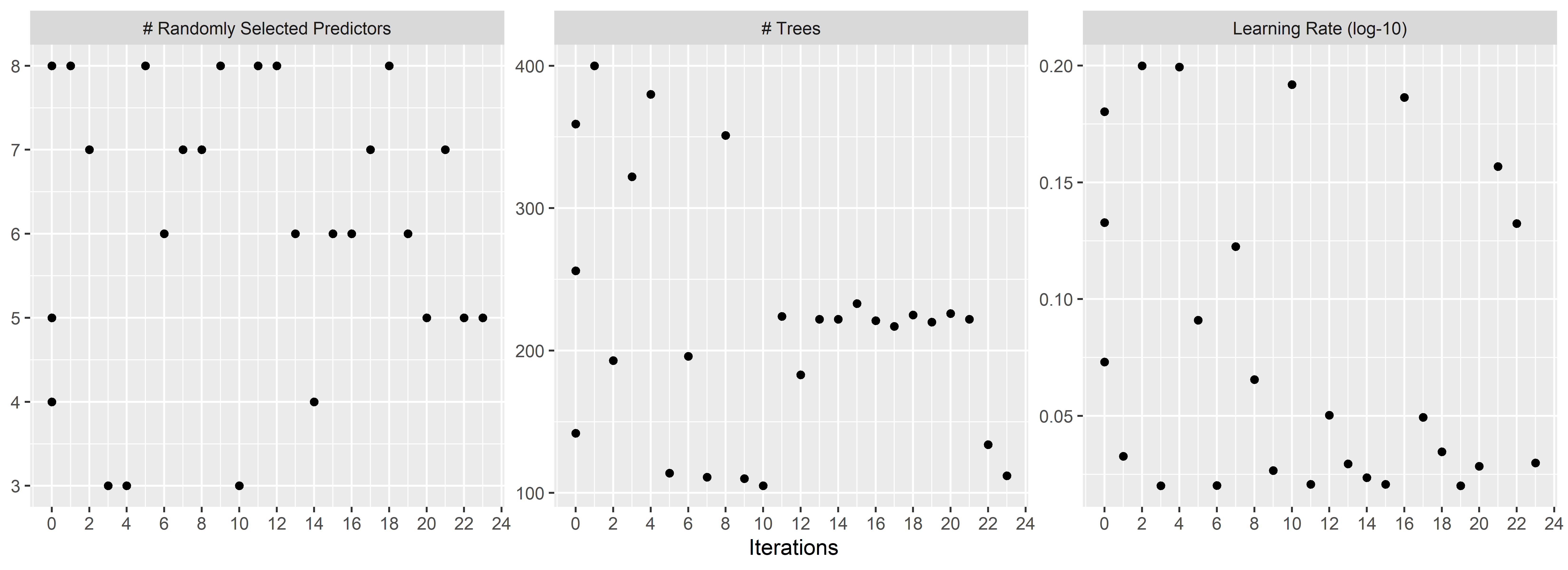
I initialize the final model using the tuned parameters from the best model ranked based on the ROC_AUC metric.
══ Workflow ════════════════════════════════════════════════════════════════════
Preprocessor: Recipe
Model: boost_tree()

── Preprocessor ────────────────────────────────────────────────────────────────
5 Recipe Steps

• step_rm()
• step_BoxCox()
• step_normalize()
• step_dummy()
• step_smote()

── Model ───────────────────────────────────────────────────────────────────────
Boosted Tree Model Specification (classification)

Main Arguments:
  mtry = 7
  trees = 217
  learn_rate = 1.12055774273203

Computational engine: xgboost
Then I evaluate the final model on the testing data from the split I performed earlier on.
          Truth
Prediction Yes  No
       Yes 190 162
No 184 871The metrics values of the accuracy and the roc_auc on the test set are respectively 75.4% and 79% as observed below.
In real life scenario, businesses need to quantify the performance of a model in a language that they can understand: money. To achieve this, I will be creating a custom metric using the yardstick package.
Over different probabilities that are inspired by the confusion matrix, our model could estimate the overall profit that it can bring to the business.
set.seed(2024)
prob_estimate <- test_results %>%
  collect_predictions() %>%
  select(Prediction_prob = .pred_Yes, Churn)

prob_estimate
# A tibble: 1,407 × 2
Prediction_prob Churn
<dbl> <fct>
1 0.763 Yes
2 0.0372 No
3 0.000232 No
4 0.00181 No
5 0.696 No
6 0.999 Yes
7 0.0444 Yes
8 0.999 Yes
9 0.000000696 No
10 0.985 Yes
# ℹ 1,397 more rowsNow, hypothetically, how much would this specific model help the company make if it was to be implemented?
I take the predictions of the model on the test set, and compare them with the truth values while using the custom metric function profit_est.
# A tibble: 1 × 3
  .metric    .estimator .estimate
  <chr>      <chr>          <dbl>
1 profit_est binary         10330
The current model can help the company earn R10 330.
What if the performance metric could be improved?
Considering the possible fluctuations of the performance of the model, below are also the possible profit that it could help the company generate.
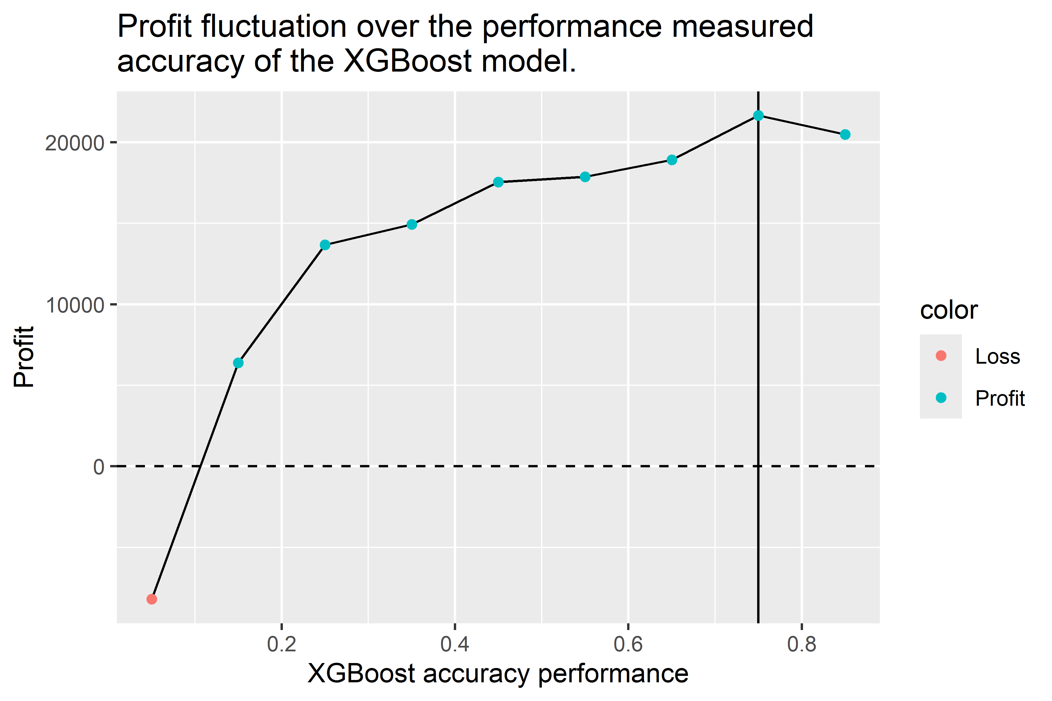
We see that an accuracy of 75% will yield the maximum profit to the company.
The XGBoost model performed quite well knowing that more techniques could be used to improve its performance among which feature selection, removing feature displaying colinearity, and increasing the number of iteration.
This is my first project for my blog website, any feedback is more than welcome.
Kelli Belcher, (2022) , Predicting Custom Churn with SMOTE .